What is Data Distillery Sip?
Sometimes, I do a livestream/blog post combo called Data Distillery Dash. I take a research topic at random1 or dataset I’ve never seen2, wrangle the data, create a predictive model or two, and write up a blog post: all within 2 hours live on Twitch! All the words and code in the part I post were written during an ~2 hour livestream. If you want to come join the party, I plan on doing this on Thursdays from 3:30-5:30 EST here.
Sometimes, I’ll want to do extensions on what I accomplished during the Data Distillery Dash, but at a (slightly) more leisurely pace. I’ve decided to call those posts Data Distillery Sips. This is the second one (see the first one here), and also serves as a continuing tutorial on how to build a predictive pipeline for psychological interventions.
Where Did We Leave Off/Why Were We Doing That?
At the end of the last post, we had explained why we needed to build two different predictive models for this particular prediction problem. Long story short, we need to generate predictions as if people had received both psychological interventions, rather than just one. For a more detailed explantion why that is, check out the previous post.
We’ve built both of those models, and we can read them in now.
We’ll also read in the holdout data we created in a previous post so we have data to make our predictions on!
holdout_ctrl <- read_rds("test_set_control.rds")
holdout_actv <- read_rds("test_set_active.rds")
Now, we’ll make predictions on each holdout set using both models. After that, we’ll wrangle the dataframes3 so they include all the info we need.
library(tidymodels)

## Apply placebo predictions within the active group

ctrl_preds_actv <- predict(ctrl_model, holdout_actv) %>%
  rename(counterfactual_pred = .pred) %>%
  bind_cols(holdout_actv %>% dplyr::select(id)) %>%
  relocate(id, everything()) %>%
  print()
# A tibble: 44 x 2
      id counterfactual_pred
   <int>               <dbl>
 1     2              0.444
 2     5              2.12
 3    10              0.0915
 4    12              1.36
 5    14              0.971
 6    15              1.22
 7    17              1.26
 8    26              1.90
 9    28              1.07
10    53              0.448
# … with 34 more rows
## Apply placebo predictions within the placebo group
ctrl_preds_ctrl <- predict(ctrl_model, holdout_ctrl) %>%
rename(received_pred = .pred) %>%
bind_cols(holdout_ctrl %>% dplyr::select(id)) %>%
relocate(id, everything()) %>%
print()
# A tibble: 49 x 2
      id received_pred
   <int>         <dbl>
 1     4         0.462
 2    24         2.54
 3    34         2.38
 4    37         0.811
 5    38         1.82
 6    47         0.693
 7    76         1.75
 8    80         1.77
 9    83         1.41
10   107         2.68
# … with 39 more rows
## Apply active predictions within the placebo group
actv_preds_ctrl <- predict(actv_model, holdout_ctrl) %>%
rename(counterfactual_pred = .pred) %>%
bind_cols(holdout_ctrl %>% dplyr::select(id)) %>%
relocate(id, everything()) %>%
print()
# A tibble: 49 x 2
      id counterfactual_pred
   <int>               <dbl>
 1     4               1.72
 2    24               2.41
 3    34               2.87
 4    37               0.978
 5    38               1.09
 6    47               0.964
 7    76               1.45
 8    80               0.898
 9    83               2.71
10   107               1.54
# … with 39 more rows
## Apply active predictions within the active group
actv_preds_actv <- predict(actv_model, holdout_actv) %>%
rename(received_pred = .pred) %>%
bind_cols(holdout_actv %>% dplyr::select(id)) %>%
relocate(id, everything()) %>%
print()
# A tibble: 44 x 2
      id received_pred
   <int>         <dbl>
 1     2        0.845
 2     5        2.23
 3    10        0.177
 4    12        0.0605
 5    14        1.37
 6    15        0.389
 7    17        1.01
 8    26        2.85
 9    28        0.912
10    53        1.70
# … with 34 more rows
We need to determine whether people were “unlucky”4 or “lucky”5 according to our models. In this case, lower scores on the SPE at timepoint 3 in the trial are the better outcome, so we’ll wrangle our data with that understanding. We also have to bring in the timepoint 06 scores on the SPE as we’ll want to make sure to control for that in our subsequent evaluation.
# Binding together the different dataframes to make our predictions about preferred intervention

ctrl_preds <- ctrl_preds_ctrl %>%
  bind_cols(actv_preds_ctrl %>% dplyr::select(counterfactual_pred)) %>%
  mutate(spe_actv_adv = received_pred - counterfactual_pred, # Higher is worse, lower is better
         prefer = factor(ifelse(spe_actv_adv > 0, "Prefer Active", "Prefer Control")),
         lucky = factor(ifelse(prefer == "Prefer Control", "Lucky", "Unlucky"))) %>%
  bind_cols(holdout_ctrl %>% dplyr::select(spe_sum_t0, spe_sum_t3)) %>%
  print()
# A tibble: 49 x 8
      id received_pred counterfactual_pr… spe_actv_adv prefer    lucky
   <int>         <dbl>              <dbl>        <dbl> <fct>     <fct>
 1     4         0.462              1.72        -1.26  Prefer C… Lucky
 2    24         2.54               2.41         0.138 Prefer A… Unlu…
 3    34         2.38               2.87        -0.492 Prefer C… Lucky
 4    37         0.811              0.978       -0.167 Prefer C… Lucky
 5    38         1.82               1.09         0.726 Prefer A… Unlu…
 6    47         0.693              0.964       -0.271 Prefer C… Lucky
 7    76         1.75               1.45         0.296 Prefer A… Unlu…
 8    80         1.77               0.898        0.876 Prefer A… Unlu…
 9    83         1.41               2.71        -1.30  Prefer C… Lucky
10   107         2.68               1.54         1.14  Prefer A… Unlu…
# … with 39 more rows, and 2 more variables: spe_sum_t0 <dbl>,
#   spe_sum_t3 <dbl>
# Now for the active condition
actv_preds <- actv_preds_actv %>%
bind_cols(ctrl_preds_actv %>% dplyr::select(counterfactual_pred)) %>%
mutate(spe_actv_adv = received_pred - counterfactual_pred, # Higher is worse, lower is better
prefer = factor(ifelse(spe_actv_adv < 0, "Prefer Active", "Prefer Control")),
lucky = factor(ifelse(prefer == "Prefer Active", "Lucky", "Unlucky"))) %>%
bind_cols(holdout_actv %>% dplyr::select(spe_sum_t0, spe_sum_t3)) %>%
print()
# A tibble: 44 x 8
      id received_pred counterfactual_pr… spe_actv_adv prefer    lucky
   <int>         <dbl>              <dbl>        <dbl> <fct>     <fct>
 1     2        0.845              0.444        0.401  Prefer C… Unlu…
 2     5        2.23               2.12         0.117  Prefer C… Unlu…
 3    10        0.177              0.0915       0.0853 Prefer C… Unlu…
 4    12        0.0605             1.36        -1.30   Prefer A… Lucky
 5    14        1.37               0.971        0.399  Prefer C… Unlu…
 6    15        0.389              1.22        -0.831  Prefer A… Lucky
 7    17        1.01               1.26        -0.246  Prefer A… Lucky
 8    26        2.85               1.90         0.954  Prefer C… Unlu…
 9    28        0.912              1.07        -0.162  Prefer A… Lucky
10    53        1.70               0.448        1.25   Prefer C… Unlu…
# … with 34 more rows, and 2 more variables: spe_sum_t0 <dbl>,
#   spe_sum_t3 <dbl>
We also see we have roughly equivalent numbers of lucky vs. unlucky participants within both intervention groups according to our models. This is a nice pattern, since it’s easier for us to believe the association between being lucky or unlucky and outcome among test set participants is due to model predictions.7
ctrl_preds %>%
  count(lucky)
# A tibble: 2 x 2
  lucky       n
  <fct>   <int>
1 Lucky      23
2 Unlucky    26
actv_preds %>%
count(lucky)
# A tibble: 2 x 2
  lucky       n
  <fct>   <int>
1 Lucky      22
2 Unlucky    22
Now, we want to see if participants in our test identified as “lucky” actually improve more than participants identified by our models as “unlucky.”
First, we make our reference level explicit in the Lucky vs. Unlucky factor variable to increase the potential interpretability of the model. In this case, we can now know that a negative coefficient for the “lucky” variable indicates lucky participants have lower/better scores on the SPE at timepoint 3 controlling for timepoint 0.8
We’re using a Bayesian model here while using default priors.9 As we can see from the summaries and plots, we can’t draw strong conclusions about whether being “lucky” according to our models actually predicted improved outcomes in the test set. With only 93 people in the holdout set the uncertainty swamps the information we have pretty substantially.
luck <- ctrl_preds %>%
  bind_rows(actv_preds) %>%
  mutate(lucky = relevel(lucky, ref = "Unlucky")) # Making Unlucky the explicit reference level

# Packages for Bayesian multiple regression

library(rstan)
library(brms)
library(psych)

# model <- brm(formula = spe_sum_t3 ~ spe_sum_t0 + lucky,
#              data    = luck,
#              seed    = 33)

# write_rds(model, "model.rds")
model <- read_rds("model.rds")
mcmc_plot(model)
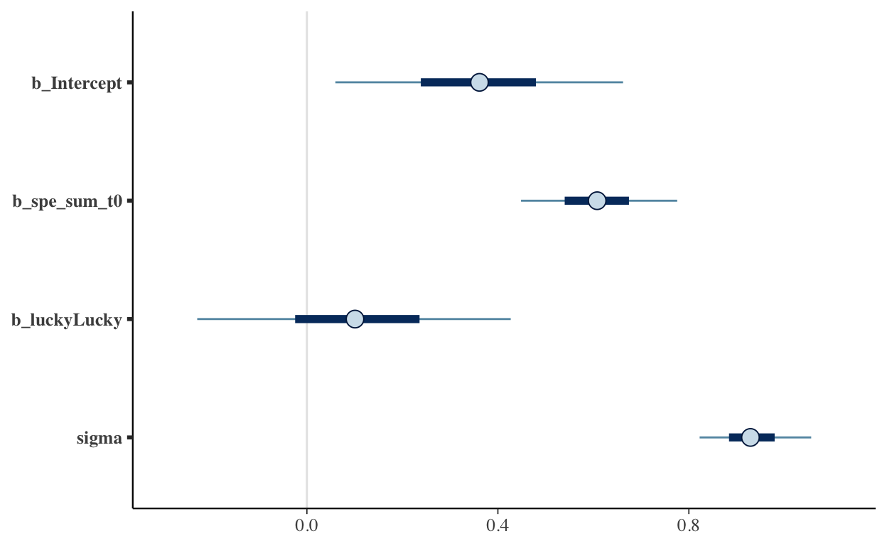
hypothesis(model, "luckyLucky < 0")
Hypothesis Tests for class b:
        Hypothesis Estimate Est.Error CI.Lower CI.Upper Evid.Ratio
1 (luckyLucky) < 0      0.1       0.2    -0.23     0.43       0.42
  Post.Prob Star
1      0.29
---
'CI': 90%-CI for one-sided and 95%-CI for two-sided hypotheses.
'*': For one-sided hypotheses, the posterior probability exceeds 95%;
for two-sided hypotheses, the value tested against lies outside the 95%-CI.
Posterior probabilities of point hypotheses assume equal prior probabilities.
Still, we now have an end to end pipeline for predicting differential response to psychological interventions! This series was for demonstration purposes only, and there are at least several ways the process could be improved.
1. Do further feature engineering to attempt to improve the models
2. Evaluating and tuning the original models more within the training sets10
3. Doing simulations to determine how many participants would be needed in the test set to overcome our uncertainty around our Lucky vs. Unlucky parameter in the final evaluation
I hope you found these posts helpful, and I’ll post more as this workflow continues to evolve.
yikes↩︎
double yikes↩︎
which the tidymodels ecosystem make super easy to create/wrangle↩︎
assigned to the intervention the model predicts would give them a worse outcome↩︎
assigned to the intervention the model predicts would give them a better outcome↩︎
baseline↩︎
and not due to some blatant confounding factor, like all the “lucky” participants being in one treatment group↩︎
baseline↩︎
we’ll dive way more into prior specification etc. for future iterations of this workflow, but since this is for demonstration we’ll keep it simpler for now↩︎
likely using workflowsets from tidymodels↩︎