Introduction:
Why Bother with Mirage Metrics?

How good is your favorite NBA team really? This is a surprisingly difficult question to answer!

I can already hear some people yelling “Scoreboard!” and pointing at readily available wins and losses for each team.

And even the most die-hard fans will admit their team sometimes gets lucky.¹ A banked 3-pointer, an untimely injury to the opposing team’s star, and so much more can make the wins and losses less reliable than they first appear.

Folks have looked at a bunch of metrics to better quantify team quality outside of luck. Average point differential per 100 possessions, the 4 factors, and many more can give us a clearer guide to how good teams are. But what if we wanted to specifically quantify how lucky they’ve been?

A precise quantification of that isn’t going to happen, at least not at scale.² But there are certain, easily measured metrics that seem to be more luck than skill-based.

Drawing on Seth Partnow’s The Midrange Theory and a myriad of Caitlin Cooper film deep-dives we’ll assume:
- Defenses don’t affect how well opponents shoot from 3 + Long 2³
- Offenses built on high-volume, very high accuracy long 2s are less sustainable than other kinds of offense⁴
- Offenses built on high-volume, unassisted high accuracy 3s are less sustainable than other kinds of offense⁵

Then, we’ll explore which 2021-2022 NBA teams may have appeared better on offense and defense than they actually were.

Load Packages

First we’ll load up the necessary packages to scrape, clean, visualize, and table our results!

Code

library(tidyverse)
library(rvest)
library(ggimage)
library(scales)
library(reactablefmtr)
library(showtext)
library(htmltools)

Scrape Data from Basketball Reference

We’ll use rvest to scrape data 2021-2022 NBA team data from Basketball Reference.

Code

html <- read_html("https://www.basketball-reference.com/leagues/NBA_2022.html")

The data we need is already in tables, so we can take advantage of that by getting all of them in just a few lines of code.

Code

bref_team_tables <- html %>% 
  html_nodes("table") %>% 
  html_table()

Tidy the Data

Now we have to tidy the data so we can visualize and table it. There are lots of little intricacies here, and feel free to explore the code chunks with their comments to learn more!

Code

# 6th table is per game opponent

per_game_opp <- data.frame(bref_team_tables[6])

# Need to redo names since R doesn't like numbers as first letter of names

per_game_names <- c("rank", "team", "g", "mp", "fg", "fga", "fg_perc",
                    "three_pointers","three_point_attempts","three_point_perc",
                    "two_pointers","two_point_attempts","two_point_perc","ft",
                    "fta","ft_perc", "orb","drb","trb","ast","stl","blk","tov",
                    "pf","pts")

# Actually assigning names to data frame

names(per_game_opp) <- per_game_names

Code

three_vs_league <- per_game_opp %>% 
  filter(team != "League Average") %>% 
  select(team, three_point_perc) %>% 
  mutate(team = str_remove(team, "\\*"),
         league_average = mean(three_point_perc),
         three_vs_league = round(three_point_perc - league_average, 4)) %>% 
  arrange(three_vs_league) %>% 
  select(team, three_vs_league)

One technique I’ve tried to use more often is keeping my cleaning notebook chunks to roughly 10-15 lines. This approach allows me to debug far more easily + think a bit more clearly about what I’m trying to accomplish at each step.

Code

# 13th table is field goal distance by opponent

shot_perc_opp <- data.frame(bref_team_tables[13]) %>% 
  select(Var.2, FG..by.Distance.4) %>% 
  filter(Var.2 != "Team") %>% 
  mutate(FG..by.Distance.4 = as.numeric(FG..by.Distance.4),
         Var.2 = str_remove(Var.2, "\\*"))

# Need to redo names since R doesn't like numbers as first letter of names

shot_perc_names <- c("team", "long_2_perc")

# Actually assigning names to data frame

names(shot_perc_opp) <- shot_perc_names

Code

# Rounding + calculating an EFG% style total metric vs. league average

opp_shot_league <- three_vs_league %>% 
  left_join(shot_perc_opp, by = "team") %>% 
  mutate(league_average = mean(long_2_perc),
         long2_vs_league = round(long_2_perc - league_average, 4),
         weighted_opp_shot = (three_vs_league * 1.5) + long2_vs_league) %>% 
  select(team, weighted_opp_shot, three_vs_league, long2_vs_league) %>% 
  arrange(weighted_opp_shot)

The end result I want is aggregated offensive + defensive mirage metrics that account for the fact that 3 points is worth 1.5 times as much as 2 points. I know that might seem obvious stated that way, but a lot of statistics don’t account for that!

Code

# 12th table is field goal distance for shooting team

shot_perc_team <- data.frame(bref_team_tables[12]) %>% 
  select(Var.2, X..of.FGA.by.Distance.4, FG..by.Distance.4,FG..by.Distance.5, X..of.FG.Ast.d.1) %>% 
  filter(Var.2 != "Team" & Var.2 != "League Average") %>% 
  mutate(
    across(
      c(X..of.FGA.by.Distance.4, FG..by.Distance.4,FG..by.Distance.5, X..of.FG.Ast.d.1),
      ~as.numeric(.x)
    ),
      Var.2 = str_remove(Var.2, "\\*"))

# Need to redo names since R doesn't like numbers as first letter of names

team_perc_names <- c("team", "long_2_volume", "long_2_perc","three_point_perc","assisted_three_perc")

# Actually assigning names to data frame

names(shot_perc_team) <- team_perc_names

Code

# Rounding + calculating an EFG% style total metric vs. league average 
# AZ-scoring since the 2 + 3 metrics are on different scales

team_shot_league <- shot_perc_team %>% 
  mutate(
    across(
      where(is.numeric),
      ~.x - mean(.x),
      .names = "vs_league_{col}"
    ),
   long2_mirage = (vs_league_long_2_volume + vs_league_long_2_perc) / 2,
   three_mirage = (three_point_perc + (1 - assisted_three_perc)) / 2
  ) %>% 
  select(team, contains("mirage")) %>% 
  mutate(across(
    where(is.numeric),
    ~scale(.x)
  ),
  weighted_team_shot = (three_mirage * 1.5 + long2_mirage) / 2) %>% 
  relocate(team, weighted_team_shot, three_mirage, long2_mirage) %>% 
  arrange(desc(weighted_team_shot))

Code

opp_shot_league <- three_vs_league %>% 
  left_join(shot_perc_opp, by = "team") %>% 
  mutate(league_average = mean(long_2_perc),
         long2_vs_league = round(long_2_perc - league_average, 4),
         weighted_opp_shot = (three_vs_league * 1.5) + long2_vs_league) %>% 
  select(team, weighted_opp_shot, three_vs_league, long2_vs_league) %>% 
  arrange(weighted_opp_shot)

Get NBA Logos for Data Visualization

I also wanted to “scrape” the logos for each NBA team for the visualizations of the Mirage Metrics later. Following Michael Lopez’s example I’m using ggimage to pull the url for each team’s logo from Wikipedia.

Code

# Get logos from Wikipedia

logos <- opp_shot_league %>% 
  select(team) %>% 
  arrange(team) %>% # Alphabetical order 
  mutate(image_url = c("https://upload.wikimedia.org/wikipedia/en/thumb/2/24/Atlanta_Hawks_logo.svg/400px-Atlanta_Hawks_logo.svg.png",
                       "https://upload.wikimedia.org/wikipedia/en/thumb/8/8f/Boston_Celtics.svg/400px-Boston_Celtics.svg.png",
                       "https://upload.wikimedia.org/wikipedia/commons/thumb/4/44/Brooklyn_Nets_newlogo.svg/340px-Brooklyn_Nets_newlogo.svg.png",
                       "https://upload.wikimedia.org/wikipedia/en/thumb/c/c4/Charlotte_Hornets_%282014%29.svg/440px-Charlotte_Hornets_%282014%29.svg.png",
                       "https://upload.wikimedia.org/wikipedia/en/thumb/6/67/Chicago_Bulls_logo.svg/400px-Chicago_Bulls_logo.svg.png",
                       "https://upload.wikimedia.org/wikipedia/commons/thumb/4/4b/Cleveland_Cavaliers_logo.svg/340px-Cleveland_Cavaliers_logo.svg.png",
                       "https://upload.wikimedia.org/wikipedia/en/thumb/9/97/Dallas_Mavericks_logo.svg/420px-Dallas_Mavericks_logo.svg.png",
                       "https://upload.wikimedia.org/wikipedia/en/thumb/7/76/Denver_Nuggets.svg/400px-Denver_Nuggets.svg.png",
                       "https://upload.wikimedia.org/wikipedia/commons/thumb/7/7c/Pistons_logo17.svg/400px-Pistons_logo17.svg.png",
                       "https://upload.wikimedia.org/wikipedia/en/thumb/0/01/Golden_State_Warriors_logo.svg/400px-Golden_State_Warriors_logo.svg.png",
                       "https://upload.wikimedia.org/wikipedia/en/thumb/2/28/Houston_Rockets.svg/340px-Houston_Rockets.svg.png",
                       "https://upload.wikimedia.org/wikipedia/en/thumb/1/1b/Indiana_Pacers.svg/400px-Indiana_Pacers.svg.png",
                       "https://upload.wikimedia.org/wikipedia/en/thumb/b/bb/Los_Angeles_Clippers_%282015%29.svg/440px-Los_Angeles_Clippers_%282015%29.svg.png",
                       "https://upload.wikimedia.org/wikipedia/commons/thumb/3/3c/Los_Angeles_Lakers_logo.svg/440px-Los_Angeles_Lakers_logo.svg.png",
                       "https://upload.wikimedia.org/wikipedia/en/thumb/f/f1/Memphis_Grizzlies.svg/380px-Memphis_Grizzlies.svg.png",
                       "https://upload.wikimedia.org/wikipedia/en/thumb/f/fb/Miami_Heat_logo.svg/400px-Miami_Heat_logo.svg.png",
                       "https://upload.wikimedia.org/wikipedia/en/thumb/4/4a/Milwaukee_Bucks_logo.svg/360px-Milwaukee_Bucks_logo.svg.png",
                       "https://upload.wikimedia.org/wikipedia/en/thumb/c/c2/Minnesota_Timberwolves_logo.svg/400px-Minnesota_Timberwolves_logo.svg.png",
                       "https://upload.wikimedia.org/wikipedia/en/thumb/0/0d/New_Orleans_Pelicans_logo.svg/460px-New_Orleans_Pelicans_logo.svg.png",
                       "https://upload.wikimedia.org/wikipedia/en/thumb/2/25/New_York_Knicks_logo.svg/480px-New_York_Knicks_logo.svg.png",
                       "https://upload.wikimedia.org/wikipedia/en/thumb/5/5d/Oklahoma_City_Thunder.svg/400px-Oklahoma_City_Thunder.svg.png",
                       "https://upload.wikimedia.org/wikipedia/en/thumb/1/10/Orlando_Magic_logo.svg/440px-Orlando_Magic_logo.svg.png",
                       "https://upload.wikimedia.org/wikipedia/en/thumb/0/0e/Philadelphia_76ers_logo.svg/400px-Philadelphia_76ers_logo.svg.png",
                       "https://upload.wikimedia.org/wikipedia/en/thumb/d/dc/Phoenix_Suns_logo.svg/380px-Phoenix_Suns_logo.svg.png",
                       "https://upload.wikimedia.org/wikipedia/en/thumb/2/21/Portland_Trail_Blazers_logo.svg/440px-Portland_Trail_Blazers_logo.svg.png",
                       "https://upload.wikimedia.org/wikipedia/en/thumb/c/c7/SacramentoKings.svg/360px-SacramentoKings.svg.png",
                       "https://upload.wikimedia.org/wikipedia/en/thumb/a/a2/San_Antonio_Spurs.svg/480px-San_Antonio_Spurs.svg.png",
                       "https://upload.wikimedia.org/wikipedia/en/thumb/3/36/Toronto_Raptors_logo.svg/400px-Toronto_Raptors_logo.svg.png",
                       "https://upload.wikimedia.org/wikipedia/en/thumb/5/52/Utah_Jazz_logo_2022.svg/460px-Utah_Jazz_logo_2022.svg.png",
                       "https://upload.wikimedia.org/wikipedia/en/thumb/0/02/Washington_Wizards_logo.svg/400px-Washington_Wizards_logo.svg.png"))

Code

# plot_labels <- tribble(~"x",~"y",~"lab_text",
#                        max(opp_shot_league$three_vs_league) - max(opp_shot_league$three_vs_league) * .125, max(opp_shot_league$long2_vs_league), "Unlucky Opp 3%, Unlucky Opp Long 2%",
#                        max(opp_shot_league$three_vs_league) - max(opp_shot_league$three_vs_league) * .125, min(opp_shot_league$long2_vs_league), "Lucky Opp 3%, Unlucky Opp Long 2%",
#                        min(opp_shot_league$three_vs_league) + max(opp_shot_league$three_vs_league) * .125, max(opp_shot_league$long2_vs_league), "Lucky Opp 3%, Unlucky Opp Long 2%",
#                        min(opp_shot_league$three_vs_league) + max(opp_shot_league$three_vs_league) * .125, min(opp_shot_league$long2_vs_league), "Lucky Opp 3%, Lucky Opp Long 2%",)

font_add_google("Graduate", "graduate")

showtext_auto()

Data Viz for Mirage Metrics

Defenstive Mirage Metrics

Code

opp_shot_league %>% 
  left_join(logos, by = "team") %>% 
  ggplot(aes(three_vs_league, long2_vs_league)) +
  geom_hline(yintercept = 0, linetype = "dashed") +
  geom_vline(xintercept = 0, linetype = "dashed") +
  geom_image(aes(image = image_url)) +
  # geom_text(data = plot_labels, aes(x, y, label = lab_text), size = 2) +
  geom_abline(slope = -2.5, intercept = seq(from = -8, to = 8, by = 4)/100, alpha = .2) +
  scale_x_reverse(label = percent) +
  scale_y_reverse(label = percent) +
  theme_minimal() +
  theme(text = element_text(family = "graduate")) +
  labs(x = "Opponent 3P% vs. League Average",
       y = "Opponent Long 2% vs. League Average",
       title = "Defensive Mirage Metrics for Full 2021-2022 NBA Season",
       caption = "Further Up & Right = More of a Mirage")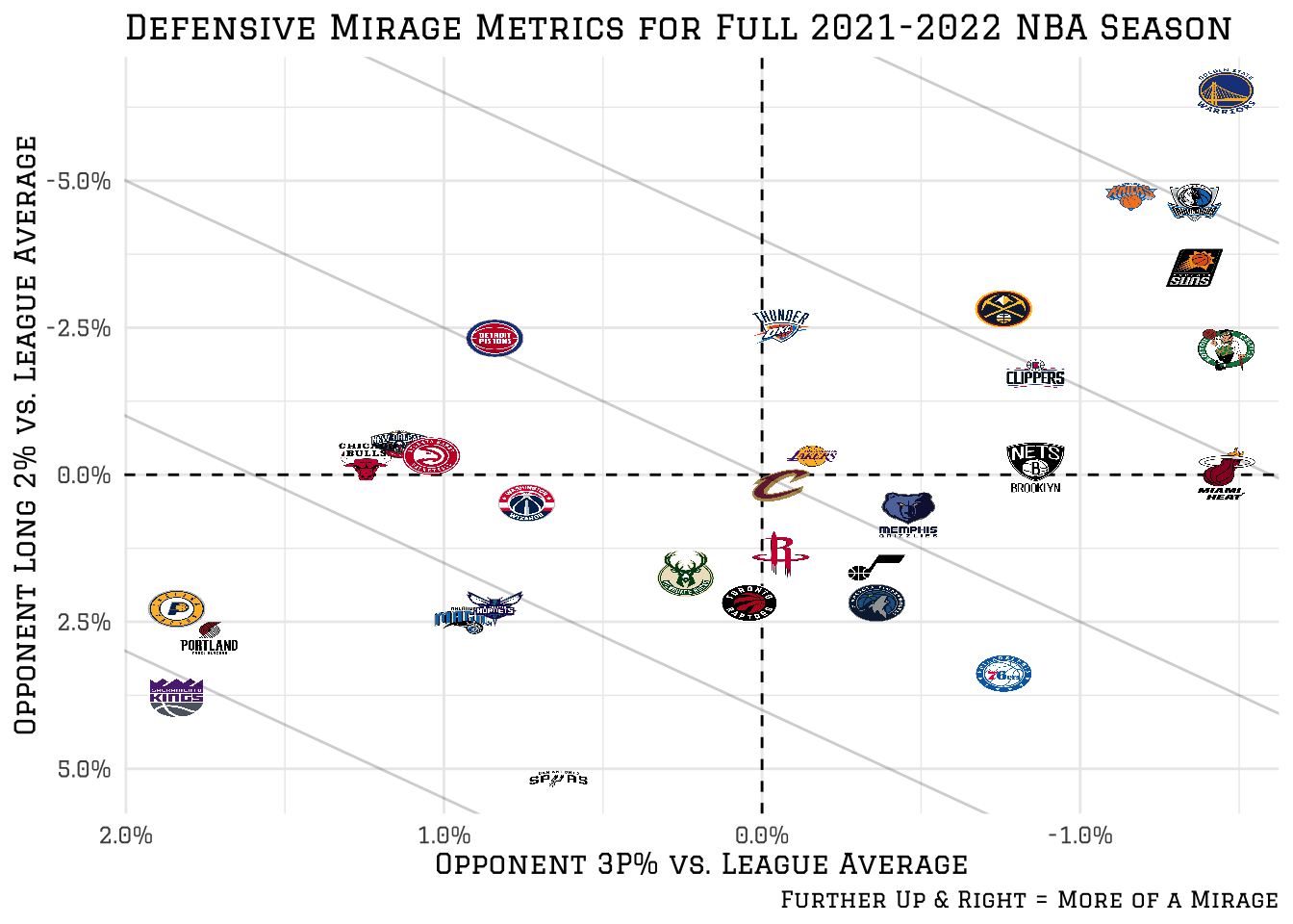

These plots take inspiration from the expected points added plots popularized via the nflfastr package by Ben Baldwin.

These plots allow us to see defensive mirage tiers rather than hard and fast rankings. I like that this plot communicates the inherent uncertainty in these metrics in an interesting way.

From a basketball perspective, we can see you need to be lucky and good to be a top defense in the NBA. I don’t think anyone would argue that the Golden State Warriors had a bad defense last year, and their already excellent defense benefitted from a lot of poor opponent shooting luck.

A couple of teams with a larger gap between “the eye test” and their defensive ratings last season also show up among the luckiest teams on defense. Put it this way: I’m not betting on either the Mavs or the Knicks having a top-tier defense again in 2022-2023.

Offensive Mirage Metrics

Code

team_shot_league %>% 
  left_join(logos, by = "team") %>% 
  ggplot(aes(three_mirage, long2_mirage)) +
  geom_hline(yintercept = 0, linetype = "dashed") +
  geom_vline(xintercept = 0, linetype = "dashed") +
  geom_image(aes(image = image_url)) +
  # geom_text(data = plot_labels, aes(x, y, label = lab_text), size = 2) +
  geom_abline(slope = -2.5, intercept = seq(from = -7.5, to = 4.5, by = 3), alpha = .2) +
  theme_minimal() +
  theme(text = element_text(family = "graduate")) +
  theme(axis.title = element_text(size = 9)) +
  labs(x = "Unassisted 3 Rate & 3P% vs. League Average - Z-Scored",
       y = "Long 2 Volume & Long 2P% vs. League Average - Z-Scored",
       title = "Offensive Mirage Metrics for Full 2021-2022 NBA Season",
       caption = "Further Up & Right = More of a Mirage")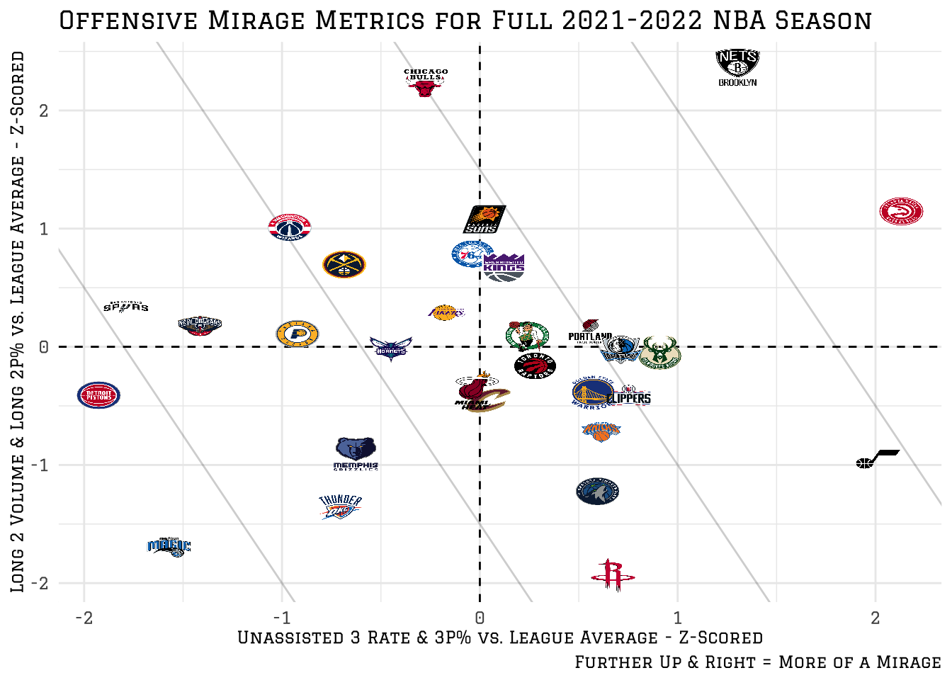

The offensive mirage statistics continue the “need to be lucky and good” story. The Atlanta Hawks had the 2nd best offensive rating in the NBA during 2021-2022, and they had an absurdly high rate of accurate, unassisted 3 pointers. You can point to all the excellent shooting Atlanta had, and also recognize that some regression to the mean is likely in 2022-2023.

Same for Brooklyn and Chicago - two teams with absurdly elite midrange shooters that might still see a bit of regression in that category this year. Case in point, the Suns are also full of elite midrange shooters and are almost a full standard deviation below Chicago on the Long 2 mirage metric.

Interactive Tables for Mirage Metrics

Additional Cleaning

As much fun as these plots are, they don’t weight 3 point luck more heavily than 2 point luck. I’ve also wanted to teach myself reactable and reactablefmtr for a bit, and this project gave me a great excuse! Shout out to Tanya Shapiro for introducing me to this package via Twitter.

Code

cleaned_table <- team_shot_league %>% 
  left_join(opp_shot_league, by = "team") %>% 
  left_join(logos, by = "team") %>% 
  mutate(across(
    c(weighted_team_shot:long2_mirage),
    ~round(.x, 1)
  ),
  across(
    c(weighted_team_shot:long2_mirage),
    ~case_when(
    .x < 0 ~ "#127852",
    .x > 0 ~  '#C40233',
    TRUE ~ '#A5A0A1'
    ),
    .names = "colors_{col}"
  ),
  across(
    c(weighted_opp_shot:long2_vs_league),
    ~case_when(
    .x < 0 ~ '#C40233',
    .x > 0 ~  "#127852",
    TRUE ~ '#A5A0A1'
    ),
    .names = "colors_{col}"
  )
  )

There was a bit more cleaning necessary to prepare the data for these tables, and I went through several iterations before settling on the current versions.

Code

initial_table <- cleaned_table %>% 
  rename(Team = team, `Total Offensive Mirage` = weighted_team_shot, 
         `Offensive Mirage 3` = three_mirage,
         `Offensive Mirage Long 2` = long2_mirage,
         `Opponent Long-Range EFG% vs. League Average` = weighted_opp_shot,
         `Opponent 3P% vs. League Average` = three_vs_league,
         `Opponent Long 2% vs. League Average` = long2_vs_league) %>% 
  relocate(image_url, Team, everything())

Huge shout-out to the extensive vignettes and documentation behind the reactablefmtr package. Going from 0 to these tables was a much smoother, more interesting process than I anticipated!

Code

off_metrics_table <- initial_table %>% 
  select(image_url, Team, contains("Offensive"),c(colors_weighted_team_shot:colors_long2_mirage))

def_metrics_table <- initial_table %>% 
  select(image_url, Team, contains("Opponent"),c(colors_weighted_opp_shot:colors_long2_vs_league))

Defensive Mirage Metrics

Code

def_metrics_table %>% 
reactable(
          pagination = FALSE,
          searchable = TRUE,
          defaultSorted = "Opponent Long-Range EFG% vs. League Average",
          style = list(fontFamily = "graduate"),
          theme = espn(centered = TRUE, header_font_size = 10, 
                       cell_padding = 7),
          columns = list(
          colors_weighted_opp_shot = colDef(show = FALSE),
          colors_three_vs_league = colDef(show = FALSE),
          colors_long2_vs_league = colDef(show = FALSE),
          image_url = colDef(
                name = "",
                maxWidth = 50,
                sortable = FALSE,
                # render team logos from their image address
                style = background_img()
              ),
          `Opponent Long-Range EFG% vs. League Average` = colDef(
            align = "center",
            cell = data_bars(initial_table,
                             text_position = "outside-base", 
                             number_fmt = percent,
                             fill_color_ref = "colors_weighted_opp_shot"
          )),
          `Opponent 3P% vs. League Average` = colDef(
            align = "center",
            cell = data_bars(initial_table,
                             text_position = "outside-base", 
                             number_fmt = percent,
                             fill_color_ref = "colors_three_vs_league"
          )),
          `Opponent Long 2% vs. League Average` = colDef(
            align = "center",
            cell = data_bars(initial_table,
                             text_position = "outside-base", 
                             number_fmt = percent,
                             fill_color_ref = "colors_long2_vs_league"
          )
          )
          )
) %>% 
    add_title(
    title = reactablefmtr::html('Defensive Mirage Metrics:<br>2021-2022 NBA Season')
  ) %>% 
  add_subtitle(
    subtitle = "Lower %s = More Mirage",
    font_size = 20,
    font_color = '#666666'
  ) %>% 
  google_font("Graduate")

Defensive Mirage Metrics:
2021-2022 NBA Season

Lower %s = More Mirage

The table matches pretty well with our earlier visualization! You can play around with the sorting by clicking on each column title or focus on your favorite team by typing it in the search bar.

Offensive Mirage Metrics

Code

reactable(off_metrics_table,
          pagination = FALSE,
          searchable = TRUE,
          defaultSortOrder = "desc",
          defaultSorted = "Total Offensive Mirage",
          style = list(fontFamily = "graduate"),
          theme = espn(centered = TRUE, header_font_size = 12, 
                       cell_padding = 7),
          columns = list(
          colors_weighted_team_shot = colDef(show = FALSE),
          colors_three_mirage = colDef(show = FALSE),
          colors_long2_mirage = colDef(show = FALSE),
          image_url = colDef(
                name = "",
                maxWidth = 50,
                sortable = FALSE,
                # render team logos from their image address
                style = background_img()
              ),
          `Total Offensive Mirage` = colDef(
      align = 'center',
      minWidth = 200,
      cell = data_bars(
        data = initial_table,
        fill_color = '#EEEEEE',
        text_position = 'outside-end',
        max_value = max(initial_table$`Total Offensive Mirage`),
        icon = 'circle',
        icon_color_ref = "colors_weighted_team_shot",
        icon_size = 15,
        text_color_ref = "colors_weighted_team_shot",
        round_edges = TRUE
      )),
      `Offensive Mirage 3` = colDef(
      align = 'center',
      minWidth = 200,
      cell = data_bars(
        data = initial_table,
        fill_color = '#EEEEEE',
        text_position = 'outside-end',
        max_value = max(initial_table$`Offensive Mirage 3`),
        icon = 'circle',
        icon_color_ref = 'colors_three_mirage',
        icon_size = 15,
        text_color_ref = 'colors_three_mirage',
        round_edges = TRUE
      )),
      `Offensive Mirage Long 2` = colDef(
      align = 'center',
      minWidth = 200,
      cell = data_bars(
        data = initial_table,
        fill_color = '#EEEEEE',
        text_position = 'outside-end',
        max_value = max(initial_table$`Offensive Mirage Long 2`),
        icon = 'circle',
        icon_color_ref = 'colors_long2_mirage',
        icon_size = 15,
        text_color_ref = 'colors_long2_mirage',
        round_edges = TRUE
      ))
          )
) %>% 
    add_title(
    title = html('Offensive Mirage Metrics:<br>2021-2022 NBA Season')
  ) %>% 
  add_subtitle(
    subtitle = html("<i class='fas fa-link'></i> Higher Numbers = More Mirage | <a href='https://www.investopedia.com/terms/z/zscore.asp'>{Metrics are Z-Scored}</a>"),
    font_size = 20,
    font_color = '#666666'
  ) %>% 
  google_font("Graduate")

Offensive Mirage Metrics:
2021-2022 NBA Season

Higher Numbers = More Mirage | {Metrics are Z-Scored}

Looking at the other end of the mirage spectrum, the Memphis Grizzlies already great-looking offense in 2021-2022 might have been held by bad luck. Counting on them to regress offensively in 2022-2023 seems like a bad bet.

On the programming side: The conditional formatting and “visualizations within tables” capabilities unlocked by reactablefmtr are fantastic. I really like gt for table building, and if I want something interactive I think I’ll default to reactablefmtr.

Conclusion

I had a lot of fun scraping, tidying, visualizing, and tabling this data! I’m also excited to formalize my understanding of which teams might be under or over-performing their actual team quality.

I’m not promising anything, and I hope to extend this initial analysis into a more extensive project at some point in the future!

If you have questions or feedback please send them my way on Twitter, and you can check out my my other data science work on my website

Footnotes

Plus even the most casual fans can regale you about the times their team has been less than lucky↩︎
I’m not going through all of last season’s film just to count the nubmer of times someone banked in a 3!↩︎
Defenses can affect accuracy at the rim + what kinds of shots teams take!↩︎
Long 2s are essentially as hard to make as 3s and it’s hard to keep up a high-accuracy on high volume↩︎
Unassisted 3s are much lower accuracy than assisted ones on average, so for a lot of teams having both metrics stay high would be really difficult↩︎

Introduction:Why Bother with Mirage Metrics?

Load Packages

Scrape Data from Basketball Reference

Tidy the Data

Get NBA Logos for Data Visualization

Data Viz for Mirage Metrics

Defenstive Mirage Metrics

Offensive Mirage Metrics

Interactive Tables for Mirage Metrics

Additional Cleaning

Defensive Mirage Metrics

Defensive Mirage Metrics:2021-2022 NBA Season

Lower %s = More Mirage

Offensive Mirage Metrics

Offensive Mirage Metrics:2021-2022 NBA Season

Higher Numbers = More Mirage | {Metrics are Z-Scored}

Conclusion

Footnotes

Introduction:
Why Bother with Mirage Metrics?

Defensive Mirage Metrics:
2021-2022 NBA Season

Offensive Mirage Metrics:
2021-2022 NBA Season